-
-
学生向け無料ソフトウェアにアクセス
Ansysは次世代の技術者を支援します
学生は、世界クラスのシミュレーションソフトウェアに無料でアクセスできます。
-
今すぐAnsysに接続!
未来をデザインする
Ansysに接続して、シミュレーションが次のブレークスルーにどのように貢献できるかを確認してください。
無料トライアル
製品およびサービス
リソースとトレーニング
当社について
Back
製品およびサービス
Ansysブログ
January 23, 2024
有限差分時間領域(FDTD)とは何ですか。
有限差分時間領域(FDTD)法は、ナノフォトニックデバイス、プロセス、および材料のモデリングに広く使用される3Dフルウェーブ電磁界ソルバーです。
フォトニクスではFDTD法が業界標準となりましたが、高周波エレクトロニクスでは有限要素法(FEM)とモーメント法(MoM)が数値電磁界ソルバーのゴールドスタンダードであり、それぞれが独自の性能を発揮しています。この記事では、特にフォトニクスシミュレーションのためのFDTD法に焦点を当てています。
FDTD法は、1966年にKane S. Yee氏によって初めて発表されました。James Clerk Maxwell氏がまとめた基礎方程式(正式には「Maxwellの方程式」と呼ばれる)を解くアルゴリズムアプローチです。19世紀に確立されたMaxwellの方程式は、電磁気学の統一をもたらし、ラジオ、テレビ、無線通信などのテクノロジーの基礎を築きました。Yeeの数値的手法は、1980年代からFDTD法と呼ばれるようになりました。
MaxwellのFDTD方程式
Maxwellの方程式とそれに付随する法則には、次のものがあります。
- 電気に関するガウスの法則: 電荷が電場を作る方法を記述した方程式
- 磁場に関するガウスの法則: 磁場が孤立した磁極を持たないことを記述した方程式
- ファラデーの電磁誘導の法則: 変化する磁場によって回路内に電磁力(EMF)がどのように誘導されるかを記述した方程式
- Ampere - Maxwellの法則: 電流を磁場に関連付け、変化する電場の役割を組み込んだ方程式
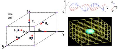
FDTD法では場の各成分はグリッドセル(Yeeセル)内のわずかに異なる位置で計算される
FDTDの仕組み
FDTD法におけるシミュレーションドメインは、シミュレーション領域によって切り捨てられ、メッシュによって離散化された空間です。FDTD法によるシミュレーションを実行すると、電磁界はすべてのメッシュセル内でMaxwellの方程式から計算され、解は時間ステップごとに変化します。空間離散化では複雑なジオメトリや構造の表現が可能になりますが、時間離散化では時間経過に伴う電磁界の変化を捉えることができます。
FDTD法の用途
FDTD法は、一般的にはオブジェクトの一部またはすべての寸法が光の波長のサイズに匹敵する設計ケースに適しています。その精度と汎用性により、FDTD法は次のようなさまざまなフォトニック設計に対応する信頼性の高いソルバーです。
- CMOS画像センサー
- LED、OLED、マイクロLED、および液晶
- 散乱および回折光学系
- メタマテリアル、メタサーフェス、メタレンズ、プラズモニクス
- 集積フォトニクス
- フォトニック結晶
FDTD法はMaxwellの方程式の最も一般的な解を示しますが、多層光学部品や回折光学部品の設計の柔軟性を最大化するなどの特定の用途には、より効率的なアプローチが適用されます。同様に、ライトガイド構造用の固有モード展開(EME)法など、フォトニクス集積素子用のソルバーの組み合わせを使用して、さまざまな構造をより効率的に処理できます。適切な問題に対して適切なソルバーを選択するための戦略的手法を確立することで、設計プロセスの速度、効率、さらには結果の精度を向上させることができます。
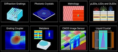
FDTD法は、さまざまなナノフォトニクス設計に使用されている
FDTDの利点
設計者は、FDTD法を使用して、さまざまな材料や構造の偏光や光の波長依存の相互作用を徹底的に解析できます。それにより、反射率、透過率、回折、干渉、吸収などの光学現象に関する知見を得ることができます。
- 時間および周波数領域の解析: FDTD法は、時間経過に伴う電磁界の変化を動的に示します。時間領域解の自動フーリエ変換が組み込まれているため、周波数解析が容易になります。
- ブロードバンド機能: 時間領域法であるため、FDTD法を使用して、単一のシミュレーションから広帯域の結果をはるかに高速に計算できます。
- 複雑なジオメトリ: FDTD法は、複雑なジオメトリのモデリングに極めて適しており、任意形状の構造を扱うことができます。
- 精度と汎用性: FDTD法は、本質的には物理的近似を行わないため、汎用性と精度に優れています。
FDTD法の課題
高い精度と汎用性を備えたFDTD法では、次のような課題があります。
- シミュレーションサイズ: 正確にモデル化できるデバイスの最大サイズは、利用できるコンピューティングリソースによって制約されます。
- シミュレーション時間:FDTD法によるシミュレーションの速度は、シミュレーションの設定や対象ボリュームから、コンピューティングシステムのハードウェア仕様まで、複数の要因に依存します。3Dシミュレーションの時間は、V . (l/dx)4の関係式でスケーリングします。ここで、Vはシミュレーションボリューム、dxはグリッドサイズです。したがって、メッシュ精度と設計サイズによって、シミュレーション時間は大きく変わります。
- メモリとコンピューティング能力: FDTD法によるシミュレーションでは、メッシュが細かくなり、シミュレーションボリュームが大きくなるにつれて、空間的および時間的な未知量の数が飛躍的に増加します。その結果、メモリとコンピューティング能力の要件が非常に高くなります。
- メモリ帯域幅: FDTD法によるシミュレーションの高速化では、特にサイズの大きいシミュレーションを扱う場合に、メモリアクセスとプロセッサ間での大量のデータ交換が課題となります。
FDTD法によるシミュレーションを高速化する方法
Ansys Lumericalでは、複数の高度なアプローチを活用してFDTD法によるシミュレーションを高速化します。
精細に調整されたアルゴリズム
LumericalのFDTDアルゴリズムは、最高レベルの精度を実現しながら計算オーバーヘッドを最小限に抑えるよう、数十年にわたって基礎レベルで微調整されてきました。メッシュ、モニター、ソース、構造、材料、解析グループなど、シミュレーション設定の効率化に役立つ特許取得済みの高度な機能を備えています。高度な最適化フレームワークが組み込まれていることで、最適化されたナノフォトニックデバイスの作成がさらに加速されます。
並列コンピューティング
Ansys Lumerical FDTDは高度に最適化された計算エンジンを搭載しており、マルチコアCPUコンピューティングシステムを活用して、ハイパフォーマンスコンピューティング(HPC)クラスタでグラフィックス処理ユニット(GPU)の並列アーキテクチャを活用できます。CPUとGPUのどちらのアーキテクチャも並列処理に優れており、FDTD法によるシミュレーションで要求される同時計算に対応します。HPCシステムでは、この並列処理を活用してワークロードを分散し、シミュレーション性能を大幅に向上させます。大規模なシミュレーションジョブは、複数の独立した計算スレッドに分割して並列に実行できるため、500~1,000億個のグリッドセルの大規模なシミュレーションでも数時間以内に完了します。
シミュレーションの複雑さが増すにつれて、効率的でスケーラブルな計算リソースが必要になります。そのような状況では、クラウドコンピューティングとHPCの組み合わせが有用となり、FDTD法によるシミュレーションを大きく変革します。Lumericalでは、CPUおよびGPUと互換性があり、オンプレミスまたはクラウド上に展開できるシミュレーションソフトウェアが提供されます。
HPCおよびクラウドのどちらにも展開できるFDTD法シミュレーションソフトウェアの詳細については、ウェビナー「HPC、GPU、およびクラウドによるフォトニック設計の高速化」をご覧ください。
基礎にあるソルバーの物理特性と、FDTD法によるシミュレーションの設定、実行、解析方法の詳細については、Ansys Innovation CoursesのFDTDラーニングトラックをご覧ください。