ANSYS BLOG
September 8, 2020
How to Optimize the Speed and Scalability of Ansys HFSS with Ansys HPC
What if you could solve complex models like a dual in-line memory (DIMM) module while preserving complete 3D electromagnetics? Or imagine solving a large 5G mmWave array antenna with fully coupled electromagnetics preserving all the finite effects of the array design.
This is all possible with Ansys HFSS and Ansys high-performance computing technologies.
Many high-frequency electronic products, including smartphones, tablet computers, software-defined radios, microwave circuits and components, active antennas and more, require multiple 3D computer-aided design (CAD) and 2D layout design tools. Traditionally it was impossible for one single electromagnetic simulation technique to solve the entire system. However, Ansys HFSS uses the latest HPC technologies so engineers can use one comprehensive electromagnetic solver to fully solve and optimize their designs.
Speeding Up HFSS Simulations
HPC is a key enabler of large-scale simulations. Matched with HFSS, HPC significantly maximizes simulation value, enabling you to increase the number of design iterations for study of larger and more complex models at faster speeds.
There are several HPC technologies that can maximize HFSS simulation speeds.
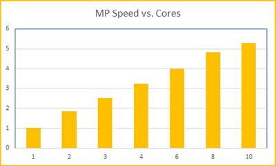
Matrix multi-processing (MP), available since 1997, is an HPC technology that uses multiple CPU cores to solve dense frontal matrices along the HFSS matrix. Each core is assigned to its own frontal matrix, allowing this portion of the solution process to speed up through parallelization. In the example below, you can expect to see an increase of up to 5X in solving speed when using 10 CPU cores.
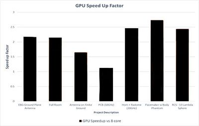
In addition to CPU matrix MP, you can leverage a graphics processing unit (GPU) for more HFSS solver speed. The GPU works in conjunction with CPUs to provide up to a 2X faster solution by applying the GPU to the largest dense frontal matrices. Only the memory required for solving the frontal matrix is needed on the GPU, therefore the overall problem size is not limited by the onboard memory of the GPU.
Keeping in mind how multiple CPUs with MP are used to solve parts of the matrix in parallel, it’s not necessary that all the memory for a problem resides on the same machine.
With the HFSS distributed memory matrix solver (DMM), you can access more memory and more cores on networked machines, so you can solve much larger problems. However, using distributed memory in no way compromises the accuracy of the solution. HFSS with DMM solves a fully coupled electromagnetic system matrix at scale.
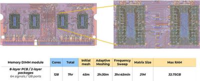
In the image below, DMM HPC and Ansys HFSS were used to solve an eight-layer, eight-module DIMM, with 128 ports across 64 signal lines. Total simulation time was only seven hours with a maximum single machine RAM of only 32.75 GB. A fully coupled, uncompromised HFSS simulation of an entire DIMM module was completed in one workday with an average RAM footprint well within the size of common compute nodes. With DMM HPC and Ansys HFSS, there is no need for large memory machines, no accuracy compromises and no uncertainty in your simulation flow.
HPC technologies can increase solver speeds while maintaining low computational costs.
Scaling Up HFSS Simulations
HFSS uses HPC capabilities to provide not only faster speeds, but also more robust network processing power to help you solve more complex, multiphysics designs.
In addition to DMM described above, there are a number of HPC capabilities that can help you maximize the scale of HFSS simulations.
Using DDM, you can break the mesh into a series of domains, which is entirely automated within HFSS. Each domain can be solved in parallel on a network computer, increasing the capacity for more cores and nodes.
In addition, DDM can efficiently solve finite-sized array antennas such as those implemented in a 5G mmWave application. Within an array structure there are common unit cells, defined as HFSS 3D Components. By defining just one of those unit cells, the 3D Component Array DDM solver virtually repeats the geometry and mesh and solves for the fully coupled antenna array.
This provides a full set of S-parameters and couplings for all the different antenna elements including coupling to other elements. In the 3D Comp Array flow, you are not limited to a single type of geometry cell but can add details such as a finite-sized ground planes or radomes, including side walls. In addition, these DDM solutions enable full-field post-processing and 3D field visualization in and about the array antenna design.
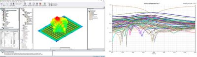
12X8 5G mmWave Antenna Array at 28 GHz, accelerated with Ansys HPC
In addition, in 2019 HFSS was deployed to the Ansys Cloud, which can be launched directly from HFSS and provides access to additional HPC hardware. This enables HFSS users to run simulations across multiple machines to solve very large problems at scale and speed. With Ansys Cloud, users have built-in, on-demand access to HPC without the burden of building a cloud environment.