-
-
Software gratuito per studenti
Ansys potenzia la nuova generazione di ingegneri
Gli studenti hanno accesso gratuito a software di simulazione di livello mondiale.
-
Connettiti subito con Ansys!
Progetta il tuo futuro
Connettiti a Ansys per scoprire come la simulazione può potenziare la tua prossima innovazione.
Customer Center
Supporto
Partner Community
Contatta l'ufficio vendite
Per Stati Uniti e Canada
Accedi
Prove Gratuite
Prodotti & Servizi
Scopri
Chi Siamo
Back
Prodotti & Servizi
Back
Scopri
Ansys potenzia la nuova generazione di ingegneri
Gli studenti hanno accesso gratuito a software di simulazione di livello mondiale.
Back
Chi Siamo
Progetta il tuo futuro
Connettiti a Ansys per scoprire come la simulazione può potenziare la tua prossima innovazione.
Customer Center
Supporto
Partner Community
Contatta l'ufficio vendite
Per Stati Uniti e Canada
Accedi
Prove Gratuite
ANSYS BLOG
November 12, 2021
Go Big with Exponential HFSS Innovation
The old adage: “If it ain’t broke, don’t fix it,” is as offensive to innovators as it is to grammarians. Just because something works well, doesn’t mean it cannot work better. As times change and technology advances, you’re either moving forward or being left behind.
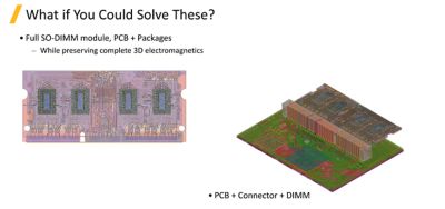
If you haven’t upgraded to the latest Ansys HFSS electromagnetic simulation software, you don’t know what you’re missing. Imagine if you could solve huge, complete electromagnetic designs while preserving the accuracy and reliability provided by HFSS. Imagine if you could solve a full SO-DIMM module, its printed circuit board (PCB) and packaging while preserving complete 3D electromagnetics. That and more is now possible with HFSS. How will that change your design methodology? How much faster will you get to market? How much better products will you deliver?
Electromagnetic Simulation Evolves
The need for speed and capacity continues to increase significantly, and HFSS has kept pace since it was released in 1990. For example, in a typical coax-to-waveguide transition the matrix size was about 10,000 elements and solving for a single frequency (the adaptive part of the simulation solution) consumed more than 10 hours. Today, the evolution of hardware has driven the need to solve huge designs, such as an anechoic chamber, and more complex designs, such as that full SO-DIMM module with its PCB and packaging mentioned earlier.
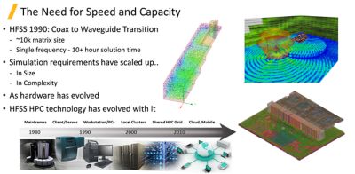
As simulation demands evolved, HFSS high-performance computing (HPC) technology has evolved right along with them to meet the demand. Desktop computers with multiple processors were introduced in the late 1990s. With this innovation, HFSS delivered Matrix Multiprocessing (MP) to enable HFSS users to simulate faster, driving faster time to market.
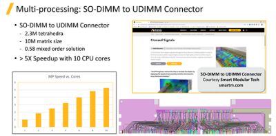
Now, HFSS leverages multiple cores at a much higher level. Individual cores solve dense frontal matrices in parallel, providing a typical 2.5x to 3x speed up over 8 cores. In a recent SO-DIMM to UDIMM Connector application, Smart Modular Tech achieved more than a 5x speed up utilizing 10 CPU cores to solve the design that had 2.3 million tetrahedra mesh elements, a matrix size of 10 million and a .58 mixed-order solution.
Graphical processing units (GPUs) turbo boost HFSS’ finite element method (FEM) solvers, providing a typical further 2x speed up. The GPU tackles the largest of the matrices. This is all easily managed by the user. Just specify the number of nodes and number of cores, and HFSS optimizes the simulation run.
MP is not limited to a single machine. The HFSS distributed memory matrix (DMM) solver provides access to more memory and cores. This enables the greatest accuracy, lowest noise floor and best efficiency for many ports with uncompromised accuracy.
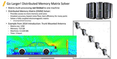
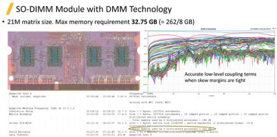
We continue to refine DMM in HFSS. In 2014, it was used to solve a trunk mounted antenna design with a matrix size of 12 million, consuming 714 GB RAM distributed over six machines (128 GB RAM per machine). Back then, this design was solved in three hours. We can now simulate an eight-layer DIMM module with two-layer packages attached to the PCB. A complex model with 64 signals and 128 ports, and a matrix size of 21 million elements was solved on Ansys Cloud. Initial meshing took 45 minutes, adaptive meshing took 2.5 hours and frequency sweep took 3.75 hours, consuming a total of 262 GB RAM. The more matrices we can solve in parallel, the more we can speed up the solution.
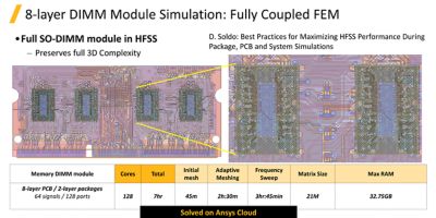
While MP speeds up the initial meshing time, we also need to speed up the remaining simulation steps. In the above figures, you can see the profile of a design created by HFSS. You can see we are using a distributed matrix solution, and the software determined that eight processors would provide the optimal resource.
If we can solve 21 million unknowns in seven hours, what else can we do? We have shattered the 100 million unknowns barrier. As a result of continuous innovation, the speed up in HFSS has been exponential, ranging from 10,000 unknowns in 1990 to over 100 million unknowns today.
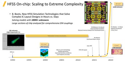
Two of the innovations that contribute to such impressive speed boosts are IC Mode, a new solver option in HFSS 3D Layout, and ECADXplorer, which improved our GDS translation.
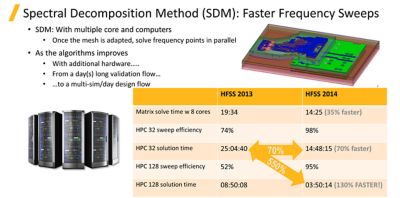
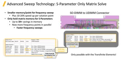
We have also sped up the frequency sweeps. Spectral Decomposition Method (SDM) allows the points in the frequency sweep to be solved in parallel. This innovation was first introduced in 2014, providing speedups of over 5x. Since then, we have continuously improved the algorithms and introduced new innovations, such as the S-Parameters Only Matrix Solve.
By providing a smaller memory point for frequency sweeps, we can achieve a 10-20% speed up per solution point. By only holding matrix memory for S-Parameters, we can achieve a 3x memory reduction, which enables you to solve more frequency points in parallel with the freed-up memory, resulting in faster frequency sweeps without compromising accuracy.
Electromagnetic Simulation Examples
Here are some examples of the simulation speed up you can expect with HFSS.
1. Package layout
A package originally simulated with HFSS 3D 2017.2, ran 2.4x faster by simply using HFSS 3D Layout. The adaptive meshing time reduced from 1 hour to 9 minutes. When using HFSS 2020 R2 3D Layout, the same package simulation ran 5.6x faster.
With every release, we are making improvements that speed up your simulations. This is a simple comparison that you can run with your own designs to show why upgrading to the latest release is well worthwhile.
2. Ground net
Another example is an entire ground net with only the critical nets simulated vs. taking a cut to simulate it. This simulation ran in about 4 hours in HFSS 2020 R2 with the cut. With the new Auto Fast setting, the entire ground structure with the critical nets takes 10 hours 24 minutes. This is a complete simulation of the design without compromise, rather than just simulating part of the design.
3. Board design
A complete board design with a cutout was simulated in HFSS 3D 2017.2 in about 18 hours. Switching to HFSS 3D Layout decreased the simulation time by 3.4x. Upgrading to HFSS 2020 R1, the design ran in 4.5 hours. By simulating on Ansys Cloud with more processors and RAM, the simulation time decreases by an additional 4.6x.
4. Crosstalk
Our final example is from Socionext. A 14-layer PAM4 package design with microvias and very tight crosstalk design requirements make crosstalk accuracy a key concern. We would typically look at critical nets and do a cutout for this to only simulate part of the design to save time. Instead, we will look at the full package.
Running on Ansys Cloud with 128 cores and 240 GB RAM distributed across eight tasks, HFSS meshes and solves the entire complex package in 18 hours.
As the Socionext example shows, as HFSS capabilities advance, so do Ansys best practices. When HFSS was limited by RAM, best practices included doing tight legacy cutouts. Now, HFSS can handle larger, simpler cutouts with similar results in run time and improved accuracy as more adjacent effects are understood. The simulation run took 68 minutes to simulate while the entire package took 7 hours, allowing you to focus on your critical nets more quickly.
Ansys continually innovates in HFSS. Each release provides faster simulation without compromising accuracy. HFSS solver technology now enables massive layout geometry handling capacity. If you haven’t used the latest HFSS, you don’t know what you’re missing.