-
-
Accédez au logiciel étudiant gratuit
Ansys donne les moyens à la prochaine génération d'ingénieurs
Les étudiants ont accès gratuitement à un logiciel de simulation de classe mondiale.
-
Connectez-vous avec Ansys maintenant !
Concevez votre avenir
Connectez-vous à Ansys pour découvrir comment la simulation peut alimenter votre prochaine percée.
Pays et régions
Espace client
Support
Communautés partenaires
Contacter le service commercial
Pour les États-Unis et le Canada
S'inscrire
Essais gratuits
Produits & Services
Apprendre
À propos d'Ansys
Back
Produits & Services
Back
Apprendre
Ansys donne les moyens à la prochaine génération d'ingénieurs
Les étudiants ont accès gratuitement à un logiciel de simulation de classe mondiale.
Back
À propos d'Ansys
Concevez votre avenir
Connectez-vous à Ansys pour découvrir comment la simulation peut alimenter votre prochaine percée.
Espace client
Support
Communautés partenaires
Contacter le service commercial
Pour les États-Unis et le Canada
S'inscrire
Essais gratuits

In the global quest for greener energy, a greener economy, and decarbonization, hydrogen and natural gas have garnered immense attention. Hydrogen is one of the most abundant elements in our universe and produces almost no pollution. This makes it an excellent candidate as an alternative to fossil fuels and can assist in decarbonizing high-emission sectors like transportation and shipping. As engineers and companies assess how to incorporate hydrogen fuel into their designs, handling these gases in a liquefied cryogenic state is an emergent interest.
However, cryogenic liquid field operations, such as storage tank filling, draining, and transportation, involve complex physics of phase change. Pervasive use of simulations has been challenging for these multiphase problems.
Let's take a look at an efficient simulation workflow to model cryogenic liquid field operations using a system-level thermal simulation tool, Ansys Thermal Desktop thermal-centric modeling software, including examples of storage tank filling, draining of liquid hydrogen (LH2), rail car transportation of liquefied natural gas (LNG), and pipeline quenching using LH2 and liquid nitrogen (LN2).
This workflow is applicable to any cryogenic liquid, such as liquid oxygen (LOX), and various refrigerants — R410a, R-32, and R-454B, to name a few.
Cryogenic Liquid Storage and Transportation Engineering Challenges
The high pressure and low temperature of a cryogenic environment presents a substantial engineering challenge for storage equipment, as well as measuring and monitoring instrumentation. The build-and-test approach is very costly and time-consuming, and increasingly engineers look to simulation to accelerate the design of storage tanks and to optimize field operations, such as filling, draining, transporting, and holding of cryogenic liquids.
Engineering design goals typically consist of:
- Minimize boil-off loss. In addition to maintaining structure integrity, the storage tanks/bottles and bulk transport containers require good insulation to minimize boil-off loss.
- Minimize cryogenic quenching liquid loss. With proper insulation, the charge/discharge pipeline between storage tanks needs to be quenched sufficiently but not overdone to avoid excessively wasting cryogenic liquid.
- Maximize filled mass. The storage tank needs to be chilled down and pressurized prior to filling. This initial state of the storage tank will affect the mass of cryogenic fluid that can be filled without exceeding structure safety limits.
Current Challenges Using 3D CFD Simulations
Simulating cryogenic fluid phase change using high-fidelity 3D computational fluid dynamics (CFD) typically requires long transient simulations that are impractical in early-stage systems design. For example, if you are simulating a filling or draining operation of the LH2 or LNG on a railcar container, it easily could take hundreds of CPU cores and days or even weeks of computation. Computationally, it’s even more time-consuming to simulate operations lasting days, such as long-distance transport or the holding/filling/draining of large industrial-scale, ground-based storage structures.
It’s clear that for these cryogenic applications, the “time to solution” may become a serious roadblock, especially during the fast-paced initial design exploration phase. To meet fast-action demands, a speedy solution pointing to correct behavior trends with big-picture input-output results is required.
An efficient simulation workflow would use the strengths from both worlds: fast system-level simulations to optimize overall design, followed by detailed CFD solutions to further optimize components and capture 3D-detailed physics where needed.
Mixed-Fidelity System-Level Simulations Solution
Among the Ansys family of solutions, Thermal Desktop software stands out with its unique mixed-fidelity system-level modeling capability. It combines 0D and 1D thermal fluid networks with 1D, 2D, and 3D solid-thermal conduction and radiation. The tool has been well known and widely used in the aerospace industry for decades.
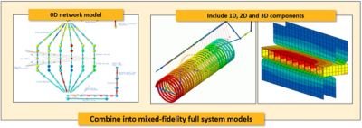
The 0D and 1D network models, combined with 2D and 3D computer-aided design bodies in a single application, allow you to create efficient system-level models.
Thermal Desktop software is equipped with a wide range of fluid properties and comes standard with the NIST REFPROF database, which is particularly useful for cryogenic applications.
The most time-consuming, computationally intensive aspect of CFD simulations is solving highly nonlinear 3D CFD equations. In Thermal Desktop software, these 3D CFD equations are replaced with nearly instantaneous solutions of 0D or 1D fluid networks, which are suited to “well-defined” flows, such as piping networks, and to account for heat transfer when the 3D details of the flow are not required.
Thermal Desktop software uses well-published empirical correlations, along with user-supplied data, for increased accuracy. For cryogenic applications, only the bulk thermodynamics effects of the cryogenic fluid are captured to interact with solid-thermal conduction. Since the latter is governed by linear equations, the whole fluid-solid thermal system can be solved very economically.
Yes, it’s fast — in fact, it’s lightning fast compared with CFD solutions, even with phase change. While gaining substantial solution speed-ups, the trade-off of a system-level solution is the lack of spatial resolution in the fluid. We would not see flow circulations, flow vectors, waves, or splashing of the liquid-gas free surface as would be the natural outcomes from a CFD simulation. Only the temporal variation of bulk quantities — mass, vapor/liquid fractions, temperature, pressure, etc. — is solved and presented.
LNG Railcar Train Ride Example
To illustrate, let’s look at a couple of typical cryogenic liquid storage tank filling/draining examples, plus a baffled LNG railcar 20-hour train ride through turns and bends, followed by a four-hour hold. These are generic models with plausible input conditions and nominal material properties to demonstrate the capabilities.
If you look closely, because we are solving for bulk temperatures, there is no temperature variation in the fluid like in a typical contour from CFD simulation. In addition, the free surface is flat as it’s simply a graphical representation of the bulk liquid/gas fractions. This ensures an incredibly fast solution time.
In the railcar train ride example, the flat free surface tilts due to acceleration when the train track bends. You would not capture waves or sloshing of the free surface, but bulk accelerations are captured. Again, the goal of a system-level simulation is to obtain fast solutions to capture the correct behavior trends sans the fluid details.
A one-hour bottom-filling event of a 30,000-gallon LNG storage tank solved in less than a minute on a single CPU core
A 20-hour train ride followed by a four-hour hold
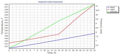
The liquid/vapor temperatures and average pressure during the 24-hour train ride
The two animations above — a 14.6-hour draining event and an 8.25-hour filling event — show a 1.25-million-gallon LH2 storage tank with a helium heat exchanger loop solved in less than 10 minutes on a single CPU core.
We love the short solution times, but how do we know if the solutions make any sense? Checks and balances come from field data, published papers, literature, high-fidelity CFD simulations — for example, from Ansys Fluent fluid simulation software or Ansys CFX CFD software — and sound engineering knowledge based on physics.
LH2 Pipeline Chill-Down Example
Next, let’s look at an LH2 pipeline chill-down example based on publicly available NIST (NBS) Report 9264. The temperature histories predicted by Thermal Desktop software show good agreement with measurement. Note the high aspect ratio (about 4,000) of the pipeline and solution time.
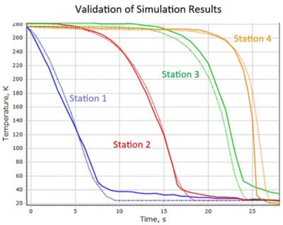
An LH2 line chill-down comparison with data. Solid lines: measured. Dotted lines: predicted.
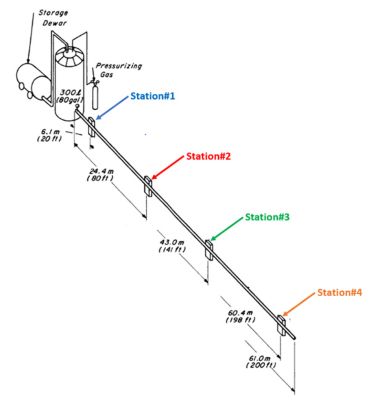
Total pipe length = 61 m. Pipe diameter = 1.5 cm.
A 28-second LH2 line chill-down event
The good agreement shown above is achieved by directly using nominal properties to fill some of the input data uncertainty gaps (see the LN2 example below) in the NIST report.
For complex problems in real life, we may not be so fortunate to easily get such close agreement from simulations. We are more likely to obtain correct trend predictions. The quality of simulation results often is plagued by input uncertainties associated with a lack of material properties or correct operating/boundary conditions. Because of that, seeing the predicted trend is good, but what if we really want the predictions to be closer to the benchmark?
Thermal Desktop software employs a lot of empirical correlations. For instance, many of the model parameters, heat transfer coefficients, and material properties can be adjusted to calibrate the solution to better approximate reality. The product features a built-in optimizer and an automated calibration routine to minimize the root-mean-square (RMS) differences between its solutions and the target from field data, literature, or high-fidelity simulations.
Let’s see an example of solution calibration. In the same NIST report, there is test data on LN2 with the same setup. Right away, the trends are good, but the results can use improvement. The main uncertainties are copper-specific heat, a frictional (pressure drop) coefficient, heat transfer coefficients, and supply pressure. By adjusting these four parameters, the temperature RMS error is reduced significantly from uncalibrated 43.8 Kelvin (K) to calibrated 12.8 K. You should not expect a perfect match, but the goal of good trend predictions and better solutions has been demonstrated all around.
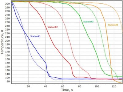
Uncalibrated solutions with a temperature RMS error of 43.8 K: An LN2 line chill-down comparison with data. Solid lines: measured. Dotted lines: predicted.
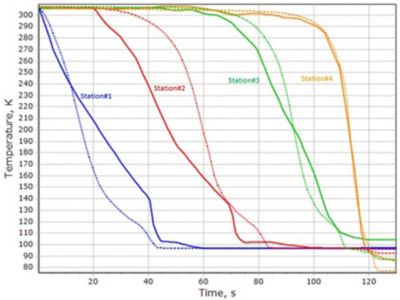
Calibrated solutions with a temperature RMS error of 12.8 K: An LN2 line chill-down comparison with data. Solid lines: measured. Dotted lines: predicted.
To avoid undue expectations, it pays to reiterate that calibration is good within reason and can go only so far. Good simulations need good data. In addition, a system-level solution inherently lacks detailed physics. Deviations from quality measurements and well-validated high-fidelity CFD solutions are to be expected.
After solving the automated calibration route, Thermal Desktop software reports and quantifies the sensitivity of RMS error relative to each of the four tuning parameters. When exploring uncharted new applications with sparse data, the product can be employed to tease out important operational parameters based on the sensitivity response of solutions. This alone can aid directional design and cut down research and development time.
Also, it might not be obvious, but we are not free from needing detailed CFD simulations. On the contrary, CFD is more of a necessity than ever. For new equipment and new process designs, there will be very little or, more likely, no data or literature to compare with. Computationally intensive it may be, but strategic use of CFD for checking/calibration and finalization, complemented by initial system-level simulations as presented here, provides an economical, competitive workflow.
Coupling Thermal Desktop Software With Fluent Software
To recap, an efficient workflow with Thermal Desktop software’s fast solutions to complement detailed CFD simulations would look like this:

In a more advanced scenario, it is also possible to co-simulate between Thermal Desktop software and Fluent software via Ansys System Coupling physics solver connection software to exchange thermal boundary information on the fly. Below shows a co-simulation of a mixing tank (fluid A) with a heating coil (fluid B). This coupling would be most beneficial, especially when the flow details are desired in the tank and with phase change inside the coil.
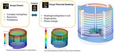
Ansys Fluent fluid simulation software and Ansys Thermal Desktop thermal-centric modeling software co-simulation of a mixing tank with two different working fluids
Learn More
Test Thermal Desktop software with a 15-day free trial, and watch this on-demand energy webinar.
The Advantage Blog
The Ansys Advantage blog, featuring contributions from Ansys and other technology experts, keeps you updated on how Ansys simulation is powering innovation that drives human advancement.


