Synopsys and Ansys power the future of innovation—connecting silicon to systems.
-
-
Access Free Student Software
Ansys empowers the next generation of engineers
Students get free access to world-class simulation software.
-
Connect with Ansys Now!
Design your future
Connect with Ansys to explore how simulation can power your next breakthrough.
Free Trials
Products & Services
Learn
About
Back
Products & Services
Back
Learn
Ansys empowers the next generation of engineers
Students get free access to world-class simulation software.
Back
About
Design your future
Connect with Ansys to explore how simulation can power your next breakthrough.
Free Trials
TOPIC DETAILS
What is Explicit Dynamics?
Explicit dynamics refers to the numerical models that represent nonlinear, dynamic behavior that use the finite element method (FEM) with an explicit time integration approach to calculate the response to applied loads over small time increments.
Explicit time integration is best suited for nonlinear problems that undergo time-dependent behavior over short durations. Typical applications for explicit dynamics analysis include drop tests, vehicle crashes, metal forming, and material failure.
Finite element analysis (FEA) simulation can also use an implicit time integration approach. The explicit approach involves many small time steps with computationally efficient calculations, but the implicit method takes fewer, larger time steps. The calculations are significantly more computationally expensive as well. Which approach is best is determined by the system's overall nonlinearity and the event's duration.
Finite Element Method
FEM is a mathematical method used to solve ordinary or partial differential equations (PDEs). For the simulation of physical systems, users break the domain into discrete chunks, referred to as finite elements, and the software applies PDEs to each element. The tool then assembles the equations, and numerical solvers are used to solve for the unknowns. Using FEM to model physical systems is called finite element analysis (FEA).
Nonlinear
In FEA, “nonlinear” refers to behavior in which the representative equation is not linear. Typical nonlinear behavior includes nonlinear material models, large deformations, boundary conditions, dynamic loading, complex contact, and material failure.
Dynamics Simulation
The full equation of motion for an object is:
Force = (mass x acceleration) + (damping x velocity) + (stiffness x deflection)
When there is minimal acceleration or the velocity is constant, a problem can be called static. In this scenario, an FEA solver only needs to determine the unknown values for force and deflection; time doesn’t play a role. However, if the velocity changes, the problem is said to be dynamic because there is change over time.
Explicit Time Integration Method
The PDEs in a finite element model representing dynamic events are solved at a given time step. Therefore, the software must integrate the PDEs over time. We call the explicit dynamics approach “explicit” because the result of the integration is an equation that explicitly calculates the value at the next time step for known quantities at the current step. The other method used in FEA, implicit time integration, is called “implicit” because the desired value at the next time step is defined only indirectly through an equation involving both known and unknown quantities. In this case, the solver uses linear algebra to calculate the implied unknowns.
One example of the explicit method, the forward Euler method, results in an equation that is only a function of the current time step:
$$y_{k+1} = y_k - \Delta t \, y_k^2 $$
Key Aspects of Explicit Dynamics Analysis
When using the explicit dynamic solution method in simulation software, both simulation beginners and experienced engineers should be aware of some important aspects of the methodology that are determined by mathematical algorithms the approach uses.
Critical Time Step and Wave Propagation Time
The most important information to consider is that the explicit solution solves for the time step just after the current time step. Because the solver calculates how strain changes over the time step, the time step size is limited to the time it takes for a strain wave to cross the smallest element in the model. This limit is called the critical time step, and how fast sound travels through the material determines the wave propagation time. For stiff materials and small element sizes, the critical time step is usually on the order of milliseconds.
Nonlinear Behavior
The next aspect engineers should be aware of is the different types of nonlinear behavior that explicit dynamics can capture. Because the explicit approach takes such small time steps, it can treat change in a calculated value over that small step as linear.
Engineers classify most nonlinear behavior in an FEA simulation into one of the following categories:
1. Nonlinear Materials
Nonlinear materials have properties that change in a nonlinear fashion due to loading or time. The most common form of material nonlinearity in almost any analysis type is plasticity. The implicit approach can have trouble with determining convergence for higher levels of plasticity, especially as material stiffness drops. Closely related to plasticity are strain rate-dependent properties such as stiffness. Another form of material nonlinearity involves abrupt changes to material properties, especially stiffness, often caused by phase changes or material failure.
2. Nonlinear Geometry
The most common form of nonlinear geometry behavior is large deformation. This is where the small strain rate formulation used in linear static analysis is no longer valid. Another form is rigid body motion, in which the body’s center of mass moves over time or the object undergoes rotation around a point.
3. Nonlinear Boundary Conditions and Loads
Convergence becomes difficult in an implicit analysis when a load changes rapidly relative to the time step. This can be an applied load or a load transmitted through contact between two bodies.
High-speed, short-duration events often exhibit these types of nonlinearities. The small time steps used in explicit time integration make it possible to approximate these changes as linear from one step to another. They also enable the solver to calculate internal forces that keep nonlinear systems in equilibrium during plasticity or material failure.
Lumped Mass Approximation
Another key aspect of the explicit time integration approach for solving dynamic problems is the ability to represent each element’s nodal mass as a lumped mass. This produces a mass matrix with a single diagonal, so the matrix inversion needed to calculate the inertial values for the model is trivial.
Quasistatic Structural Analysis
A subset of dynamic structural analysis occurs when the inertial effects in a system are small enough to be ignored, and the system remains essentially in equilibrium the entire time. A good example of this type of behavior is metal forming. It is dynamic in that the material properties, especially plasticity, are time dependent, but the inertia of the metal doesn’t impact its plastic deformation.
What is Implicit Dynamics?
It is difficult to talk about explicit dynamics without discussing implicit dynamics. As the name implies, implicit dynamics is an FEA simulation approach that uses an implicit time integration scheme. Like explicit dynamics, implicit dynamics still solves the full equation of motion over time with multiple time steps.
The equations for the implicit integration method involve values for both the current time step and the next time step. For implicit simulation software tools, the solver uses a backward Euler method to derive equations for a value at the next time step that are a function of the current step (k) and the next time step:
$$y_{k+1} = \frac{-1 + \sqrt{1 + 4 \Delta t y_k}}{2 \Delta t} $$
The Difference Between the Implicit Method and Explicit Methods
Engineers use both integration approaches in structural analysis for dynamic and quasistatic simulations. As mentioned in the introduction, the primary difference is that when the PDEs are integrated in the explicit method, the solution is fully defined by the resulting equation. In the implicit method, the unknown values are implied, so the algorithm must use linear algebra to find the solution.
From a real-world, practical perspective, this results in the following differences:
| Implicit Method | Explicit Method | |
| Time Step Size | Set by user to capture changes in load and assist nonlinear calculations to converge. The time step is large, requiring very few steps. | Set by wave propagation time across the smallest element in the mesh. Time step size is on the order of milliseconds, requiring many steps even for short durations. |
| Compute Cycles Per Step | Full solution of simultaneous equations. Multiple solves per time step if nonlinear calculations need to converge. | Very efficient, explicit solution for each step with easily inverted lumped mass. |
| Memory Requirements | The implicit integration method and full mass matrix require significantly more memory than explicit methods. | The explicit integration method and lumped mass formulation require much less memory than implicit methods. |
| Convergence | Convergence must be achieved at each time step for nonlinear calculations, establishing equilibrium. | Not needed because a small time step allows for linear assumption. |
| Equilibrium | Required | Not required |
| Mesh Count Sensitivity for Compute Resources | Problem dependent because the resulting matrix bandwidth drives solve times. | Linearly dependent on the number of elements. |
| Element Size Sensitivity | Runtime is relatively independent of the size of individual elements. | Linearly dependent on the smallest element size. Halving the smallest element doubles the runtime. |
| Contact | Must iterate until force equilibrium is achieved. The solution can diverge if abrupt contact changes occur. | No iteration required. Handles abrupt contact changes well. |
| Material Failure | Removing element stiffness or the connection between elements can result in convergence issues and often requires adaptive meshing. | Handled smoothly because of the small time step. |
| Material nonlinearities | Abrupt changes in properties and low stiffness can cause equilibrium problems and, therefore, convergence issues. | A small time step allows for linear treatment in a given time step. |
Examples of Explicit Dynamics Simulation
The small time step size and lumped mass formulation used in explicit dynamics analysis make it ideal for short-duration events with significant nonlinearities. Users may choose this approach over implicit analysis for longer, quasistatic events with equilibrium issues.
Engineers can use Ansys explicit dynamics solutions like Ansys LS-DYNA software, across industries to quickly generate useful information for highly complex, nonlinear structural simulations. Below is a list of some of the more common applications.
Drop Testing
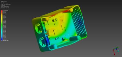
Both consumer and industry products need to survive drops from a reasonable height during shipping and use, so engineers use industry standards for drop testing to ensure their products are sufficiently robust. But doing physical tests is expensive and require real hardware. Using a tool like LS-DYNA software that can connect to computer-aided design (CAD) models through the Ansys Workbench platform reduces the cost and moves virtual drop testing to an earlier, less expensive part of the product development process.
Vehicle Impact

Of all the applications of explicit dynamics simulation, car crash analysis and simulation has likely affected the most people and saved countless lives. A vehicle impact into a solid object or another vehicle involves the crushing and failure of metal structures over a short period of time — an ideal application for explicit dynamics. That is why all vehicle manufacturers simulate full vehicles, seat belt systems, airbags, and battery packs using an application like LS-DYNA software or similar software tools.
Human Body Impact

Short-duration events that impart force to an object occur not only with products and machines, but they also impact the human body. For this reason, engineers include high-fidelity, structural human body models like the Ansys Hans model in their explicit dynamics simulations. No longer just a dummy representing shape and mass, a detailed human structural model can show the loads and areas of injury to any part of the human anatomy in a variety of situations, from race car collisions to a punch to the head.
Heart Simulation
The human heart is one of the most complex examples of structurally driven multiphysics. Electrical impulses trigger large deformations in muscle tissues, which in turn push and pull blood through valves that open and close. Researchers and engineers model this dynamic interaction, including the computational fluid dynamics (CFD) of parts like blood flow, in a true multiphysics explicit dynamics tool like LS-DYNA software.
Metal Forming
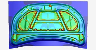
Humans have been pounding metal into shape since the Bronze Age, but in the Silicon Age, we use explicit dynamics simulation to optimize the process. The forming stage, in which a rigid tool bends and shapes thin sheets of metal, is an ideal application for the explicit dynamics method in FEA. In contrast, processes like springback and heat treating are longer in duration and are best solved through implicit analysis. Because of this, engineers can use a workflow that either moves the simulation from an explicit tool like LS-DYNA software to the implicit solver in the same tool or to a separate software application like Ansys Mechanical structural FEA software.
Solder Reflow
Semiconductor manufacturers produce millions of microchips yearly that use tiny balls of solder to physically and electrically connect the chips. The quality of these solder balls impacts the performance, cooling, and robustness of nearly every electronics product. Explicit dynamics simulation can handle the highly nonlinear material behavior of the solder as it melts, flows under surface tension, and then solidifies.
These are just a few of the more common applications of explicit dynamics software tools. Other uses include:
- Defense applications, especially those involving munitions and armor. Ansys Autodyn software is an especially good tool for this class of problems.
- Machining processes like milling and turning to optimize tool design and machining speed
- Sloshing behavior in containers as vehicles maneuver
- Buckling of structures under critical loads
- Sporting goods products subjected to short, dynamic events
Advances in solver capability, user interfaces, and computing power have greatly expanded the use of explicit dynamics. Once limited to high-end aerospace and defense (A&D) applications, this method is now used in automotive design and many other fields. It is particularly valuable in situations involving short but intense loading or nonlinearities that traditional implicit time integration solvers struggle to handle.
Leading vendors like Ansys also provide extensive training, support, and examples to help engineers become proficient and drive their designs to achieve increased performance, greater safety, and improved durability.
Related Resources
Let’s Get Started
If you're facing engineering challenges, our team is here to assist. With a wealth of experience and a commitment to innovation, we invite you to reach out to us. Let's collaborate to turn your engineering obstacles into opportunities for growth and success. Contact us today to start the conversation.