-
-
Access Free Student Software
Ansys empowers the next generation of engineers
Students get free access to world-class simulation software.
-
Connect with Ansys Now!
Design your future
Connect with Ansys to explore how simulation can power your next breakthrough.
Countries & Regions
Free Trials
Products & Services
Learn
About
Back
Products & Services
Back
Learn
Ansys empowers the next generation of engineers
Students get free access to world-class simulation software.
Back
About
Design your future
Connect with Ansys to explore how simulation can power your next breakthrough.
Free Trials
ANSYS BLOG
February 28, 2023
Application-Specific Parameter Changes to Maximize the Perception of Simulation Results in Ansys Zemax and Speos
As a leader in the automotive lighting space, we wanted to share some advice on how to maximize the benefits of our simulation software. By adjusting parameters to best fit your application area, you’re doing more to create the right conditions for confidence-based design.
Through customer questions, we’ll explore parameter changes to maximize the perception of your simulation results in the context of an exterior automotive lighting example: a rear lamp model in Ansys Speos.
What Factor has the Most Influence Over the Quality and Speed of my Simulation?
The sensor. Appropriate sensor settings can dramatically change your simulation results. If you’ve gone through the effort of building a physically accurate, high-fidelity model, make sure you’re taking advantage of everything the model has to offer. If you’re viewing results with 1080-pixel resolution on a 4K monitor, there’s going to be noticeable pixelation and lack of sharpness. Unless you’re looking for a quick, low-fidelity image, don’t reduce the resolution of your results and lose out on quality.
Sampling is the main parameter you want to look out for. Higher sampling means a smoother, more beautiful result, but it does require longer simulation time. For example, if you double X and Y sampling in Figure 1, you need four times as much simulation time to get your results.
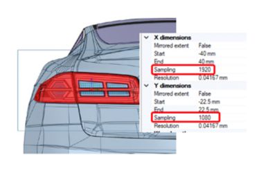
Figure 1: Sampling settings for smoother simulation results.
A few reminders:
- A “smooth” result is a minimum of 1920 pixels (i.e., sampling) for the longer side of the sensor.
- For square pixels, the resolution of the shorter side of the sensor should be the same as the longer side.
- If you’re magnifying results by zooming in, your sampling should be around 4,000 pixels, so results remain smooth under magnified conditions.
- In the case of radiance sensors, we’d recommend positioning the frame as close as possible to the object (lamp) and as far as possible from the eye point to achieve a large focal distance.
What Settings can I Change to Enhance the Mesh Quality of my Simulation?
In a physical assembly, all components are physically attached or manufactured (e.g., overmolded) with some degree of tangency. The computer-aided design (CAD) data used for Speos simulation is tessellated according to the defined meshing settings; thus, the original accuracy of the CAD model changes. A fine mesh is critical to reduce the artifacts caused by volume conflict and/or gaps (Figure 2).
There are specific options, settings, and parameters that can help you make the most out of your simulation. Default parameters work well, but if you have a large error during simulation (i.e., over 10%), you should change geometrical tolerances. Large error is most common in LED geometries and other miniature geometries. If you run your simulation, and you’re still getting large errors or unexpected gaps, you may adjust the meshing sag value and/or meshing step value down to a fixed 0.01 millimeter value.
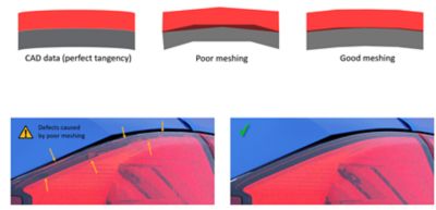
Figure 2: In physical assemblies, a fine mesh reduces the artifacts caused by volume conflict and/or gaps.
When using a light guide or diffusing material that may generate many impacts, increase the maximum number of surface interactions up to 1,000 by right-clicking on Simulation > Options > Simulation.
Which Simulation Type do you Recommend: Direct or Inverse?
In short, we recommend running both direct and inverse simulation, as they both have their advantages.
When attempting to evaluate a lamp’s lit appearance, the sensor is typically located at a position where many rays are passing through. Under those conditions, direct simulation is a faster method for collecting rays and achieving results with less noise. Direct simulation is also advantageous because you can use multiple sensors in a single simulation without increasing the simulation time. That’s not the case in an inverse simulation because simulation time is multiplied by the number of sensors.
In each pass, inverse simulation generates rays between a focal point on the sensor and each pixel on the front face. If the sensor covers a large area outside of the lamp, many rays won’t contribute to the lit appearance. In cases where the sensor is small and covers the area of the lamp, inverse simulation can be as efficient as direct simulation. That said, in vehicle design, the sensor is typically made to contain the car body and background.
What are the Most Advantageous Settings for Direct Simulation?
Gathering
Gathering improves simulation performance by enabling sensor gathering and improving the convergence rate for radiance or luminance sensors. Gathering is a dedicated parameter and not editable, but it’s always active.
Integration Angle
Gathering can’t provide the same benefits with a specular surface, so an integration cone is recommended for some approximation. If the angular deviation from the ray toward the focal point (“virtual ray” in Figure 3) is less than the integration angle, the ray reaches the focal point. If the integration angle is too large, rays converge faster, but the results are blurry. If the integration angle is too small, rays converge slower, but results are more accurate.
A two-degree integration angle is usually a good value for most automotive lighting applications. It should, however, be evaluated to find the best quality-computation time trade-off.
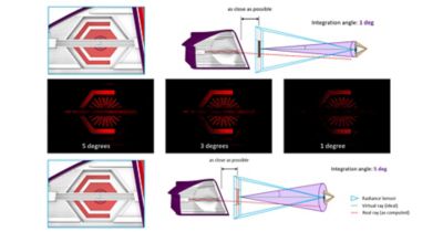
Figure 3: Comparing simulation output at different integration angles.
Fast Transmission Gathering (FTG)
Automotive lamps always have an outer lens with a specular surface, so gathering is canceled at the impact on the outer lens and rays are calculated with the integration cone. Optical components like reflectors have a specular optical property, too. If there’s an outer lens in the design, the integration cone is calculated at the outer lens, often with blurry results. This can be remedied by reducing the integration angle; however, simulation will take longer without using FTG.
To maintain gathering and integration angle, enable FTG. FTG allows the rays to ignore the refraction on the outer lens. So long as the outer lens is made of parallel surfaces with consistent thicknesses, ignoring refraction has little impact on accuracy. Reflection and absorption on the lens are still considered.
Once I’ve Completed Sensor Setup and Selected Simulation Options, how Long do I run my Simulation?
In Figure 4 below, you’ll find length guidelines for inverse and direct simulations. In the case of a direct simulation, rays are a metric for defining how long a simulation can run; with more rays, you’ll have a higher-fidelity model. Below, we provide guidance for a rough study (i.e., during design iterations), quick review (i.e., after a semi-major milestone), and detailed review (i.e., in the design validation stage). Performing these reviews will inspire confidence in a design’s ability to meet requirements and quality standards.
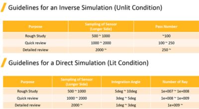
Figure 4: Guidelines for inverse (top) and direct (bottom) simulation, broken down by design phase.
Now That I Have Direct and Inverse Simulation Results, how can I Make Best use of Them?
We’d recommend running a separate simulation for each function (i.e., tail/stop, turn indicator, reversing, etc.) and then uniting your results using the map union operation of photometric calc (Figure 5). Hint: You can select multiple files at once; no need to only unite two at a time.
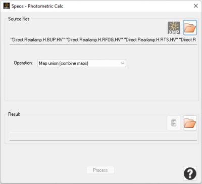
Figure 5: Window allowing you to unite separate simulation results using the map union operation.
This approach also saves time in the event a function is modified. There’s no need to rerun your consolidated simulation, so just replace the old function with the new one (Figure 6).
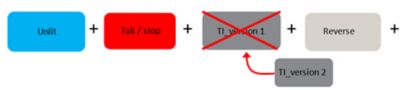
Figure 6: Method for creating a total result when one of many functions is modified.
Remember, rays are distributed based on the ratio of source flux, so if you make a single simulation that includes all functions, the function with a smaller flux receives fewer rays than the others (e.g., tail). We avoid this by simulating each function independently and uniting the separate functions. See Figure 7 for an example output.
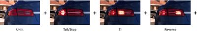
Figure 7: Output of simulating separate functions and uniting them.
What Post-Processing Settings Should I Implement Once I Have Results?
Color Management
It is important to implement settings that optimize the color accuracy and saturation of the monitor on which you’re viewing the results. As shown in Figure 8, a standard monitor may only capture a small portion of the color spectrum. If the red color of your rear lamp is outside of that area, image results appear more saturated than they really are because the monitor lacks the ability to display results accurately.
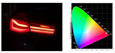
Figure 8: The area inside the triangle represents what the computer monitor can display (right); the “X” outside the triangle marks the red color of the rear lamp (left).
For tail and stop lamps, we recommend selecting maintain lightness and hue because of the relatively high dynamic range. See Figure 9 for a visual representation of all three-color space conversion options in Speos.
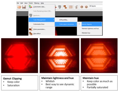
Figure 9: A side-by-side comparison of color space conversion options and their impact on how simulation results are perceived.
Adaptation
The human eye must adapt to the luminance level of the environment. Adaptation considers the capabilities of your display and adjusts the gradient of the displayed luminance values. The goal is to either (a) accommodate a specified luminance value (i.e., local adaptation), or (b) mimic the spatial adaptation of the eye as it scans different regions of the map. The linear scale of a luminance map in the Ansys Photometric Lab doesn’t have this capability.
The dynamic adaptation 2019 type setting is best practice when your sensor has a wide field of view (similar to our actual eyes) so the overall luminance is properly considered. When the sensor has a narrow field of view, local adaptation is preferred. That way, the overall luminance can be set manually, since the reduced field of view contains only a fraction of the overall luminance a real eye would see (Figure 10).
Glare
The Holladay, 1926 glare effect setting offers a faster, simpler calculation; however, given computing capabilities today, Vos, 1984 is our recommended setting (Figure 10). If your model has noise (e.g., pixels with high luminance), Vos, 1984 may generate an undesired sparkling effect. To negate this effect, you should always include an environmental light source, even if it’s a low level of light. In parallel, increasing the number of rays will also help eliminate noise. If you’re short on time, use Holladay, 1926 instead to show brightness in a realistic manner.
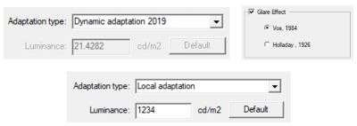
Figure 10: Preferred adaption and glare settings in the Ansys Virtual Human Vision Lab.
Vision Mode Evaluation
We’d recommend that your vision mode evaluation is based on maximum value of the xmp (Figure 11). Maximum value is best for nighttime driving conditions or other low luminance scenarios because average value can be low, resulting in mesopic or scotopic vision.
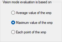
Figure 11: Vision mode evaluation settings in the Ansys Virtual Human Vision Lab.
What Should my Results Look Like?
These are the results you can expect by following the best practices we’ve covered here (Figure 12). If you’re interested in hands-on experimentation, you can access this model through our tutorial. Try it for yourself here.
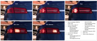
Figure 12: Simulation results when all suggested parameters are implemented.