


TOPIC DETAILS
What is Computational Fluid Dynamics (CFD)?
Computational fluid dynamics (CFD) is the science of using computers to predict liquid and gas flows based on the governing equations of conservation of mass, momentum, and energy. Fluids are all around us and sustain our lives in endless ways. The vibrations in your vocal cords generate pressure waves in the air that make speech possible, as well as hearing the spoken words. Without fluids, your tennis ball’s topspin would be meaningless, and your airplane wouldn’t generate any lift. Through CFD, we can analyze, understand, and predict the fluids that make up nearly every part of our world.
Examples of Computational Fluid Dynamics
CFD is used wherever there is a need to predict fluid flow and heat transfer, or to understand the effects of fluid flow on a product or system. CFD analyzes different properties of fluid flow, such as temperature, pressure, velocity, and density, and can be applied to a broad range of engineering problems across industries, including:
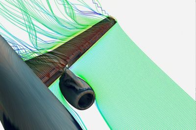
Aerospace and Defense: CFD makes it possible to model the airflow around aircraft to predict lift and drag, known as external aerodynamics. This is important as companies look to optimize aircraft designs for improved performance and decreased fuel usage. CFD can also simulate complex systems within the aircraft's interior, such as cabin air circulation, to predict air quality. Key applications include Avionics cooling, aero-optics, external aerodynamics, cabin HVAC, and propulsion.
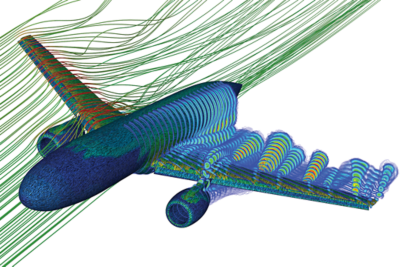
Ansys Fluent simulation of an external aerodynamics study of a commercial aircraft.
Automotive: In electric vehicles, where e-motors and battery electrochemistry create complex intersections between mechanical, chemical, and electrical engineering, CFD allows us to conduct detailed thermal studies throughout the multiphysics system. This can help engineers predict how efficiently the motor is cooled and reduce battery thermal runaway that can cause fires. Key applications include gearbox lubrication, autonomous sensors, aeroacoustics, external aerodynamics, battery modeling, and electric motor cooling.
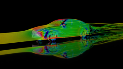
A Driver model solved using the Ansys Fluent GPU solver
New Energy: As an enabler for decarbonization, hydrogen is a valuable fuel in creating a cleaner planet. CFD allows us to model the full hydrogen value chain—from production to storage, transportation, and consumption. CFD can conduct exploratory studies to learn how hydrogen and other alternative fuels can be used in conventional engines and determine the efficacy of alternative fuel options. Key applications include PEM electrolysis, hydrogen production, transportation, storage, and consumption, and fuel cell utilization.
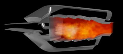
A combustion study performed in Ansys Fluent
Healthcare: In the biomedical field, CFD can analyze fluid flows in the human body, such as blood flow through the circulatory system and airflow through the respiratory system. It can also be used to speed the development of medical devices and evaluate the potential efficacy of new medications. Key applications include cardiovascular flow, respiratory system, biopharmaceuticals.
How Computational Fluid Dynamics Works
There are many different approaches to solving fluid flow on a computer. Before you start, you need to determine what methodology you will use at a high level, i.e., what governing equations will be solved. This choice will narrow down which computational approaches are available. Assuming a continuum approach is chosen (which is quite common), there are essentially 3 steps.
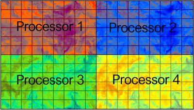
First, the fluid flow domain (the continuous region to be calculated), is identified (typically represented by a CAD model). Then, a mesh is applied to dissect the domain into well-defined cells. Finally, the discretized version of the governing fluid equations is solved by the computer within each cell. In the context of high-performance computing (HPC), an optional step is assigning different cell groups to different computers for parallel processing.
1. Identify the fluid flow domain to be solved
2. Discretize the domain into the desired mesh size and grid spacing

2. Assign processors to different regions and apply the appropriate calculus equations
Challenges of Modeling Fluid Flow
The complicated nature of fluid flow makes modeling it on a computer inherently difficult. Multiphysics interactions, nonlinearity, and unsteadiness are some of the complexities that make analyzing fluids so challenging.
Multiphysics interactions: Fluids don’t usually flow in isolation: they flow within, through, and around structures. Think about trees moving in the wind. When the tree moves it changes the wind, and the wind changes the tree. This coupled problem of fluid interacting with a structure requires a multiphysics approach to modeling.
Ansys CFD software, such as Fluent and LS-Dyna, can solve fluid-structure interaction problems like this (sometimes coupling with a structural mechanics solver, like Ansys Mechanical). And even when considering the fluid in isolation, many real-world scenarios involve multiple fluids (e.g., air bubbles rising through water) and/or changes to the chemical composition of a fluid through reactions (e.g., combusting flow inside an aircraft engine or the chemical reactions occurring in your car’s battery). Ansys Fluent is particularly well-suited to model these situations.
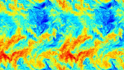
Nonlinearity: In fluid dynamics, this property of the governing physical equations means that the fluid interacts with itself. Most flows of engineering interest are turbulent in nature. Turbulence is one example of a nonlinearity in fluid dynamics, since turbulence affects other quantities like heat transfer and momentum, which in turn affect turbulence. By turbulence (yes, like what the captain is talking about on the airplane), we mean that the flow is random, chaotic, and non-deterministic.
This randomness is why a key component of computational fluid dynamics is the word “computational.” Because of nonlinearity and turbulence, there’s no pencil-to-paper way to solve these equations. It must be done on a computer (save for a few simple laminar flows with low dimensionality). Even then, the answer to a CFD problem is not a solution—it’s the computer’s calculated solution after turning a bunch of calculus into algebra.
Unsteadiness: An inherent feature of turbulence is unsteadiness. This means that the flow quantities at any fixed point in space change with time. If this unsteadiness is significant (e.g., your car driving on the highway), a highly accurate simulation requires a time-resolved solution, which greatly increases the cost.
The widespread phenomenon of turbulence has stumped scientists and engineers for generations. It is so complicated that Nobel Prize-winning theoretical physicist Richard Feynman called it “the most important unsolved problem of classical physics.”. While CFD doesn’t solve the problem of turbulence from a mathematical perspective, it allows engineers to create models that account for the effects of turbulence in their designs.
History of Computational Fluid Dynamics
The study of computational fluid dynamics started in the early 20th century when mathematical models were first developed to address fluid flow. As computers emerged in the mid-20th century, the field quickly evolved thanks to their calculation speed and ability to model increasingly complex problems.
Early development (1900s-1940s):
The basic governing equations for fluid flow, known as the Navier-Stokes equations, are developed. These equations provide the theoretical framework for understanding fluid behavior.
Computers emerge (1950s-1960s):
This turning point in CFD made it possible to perform complex calculations at high speed and get answers to fluid flow problems once considered impossible to solve.
Numerical methods (1960s-1970s):
Applying numerical methods gave researchers the ability to divide a domain into a grid of smaller elements to solve for fluid properties within each element. This allowed for more complex geometries and boundary conditions to be analyzed.
High-Performance Computing (HPC) (2000s-Present):
With advancements in HPC, running larger, more complex CFD models in less time is possible. The massive processing power of HPC allows engineers to perform extremely large computations on complex processes, such as analyzing a whole aircraft in flight.
Governing Equations of CFD
The motion of fluid is not intuitive for many people, as it moves very differently than a solid object. If you throw a ball across the room, it doesn’t change shape or mass. You can’t quite “throw” air in the same way. The governing equations of CFD help us compensate for the arbitrary shape and unpredictable nature of fluids.
The Navier-Stokes equations, named after Claude-Louis Navier and George Gabriel Stokes, are partial differential equations describing the motion of fluids. Developed in the mid-19th century, they are the basic equations for understanding fluid mechanics and are used to model all types of fluid flows, such as airflow around a wing and fuel flow through an engine. They are considered the primary governing equations for modeling fluid behavior, and are based on the conservation equations for mass, momentum, and energy.
1. Conservation of Mass: Continuity Equation
This equation states that the mass of a given volume of fluid must remain constant unless there is a mass inflow or outflow:
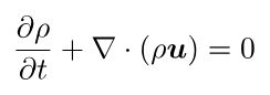
Where ⍴ is the fluid density, t is time, u the velocity vector and ∇ the gradient operator.
2. Conservation of Momentum: Newton’s Second Law
The momentum equation states that the rate of change of momentum within a fluid volume is equal to the sum of the forces acting on it, including pressure and gravity. For an incompressible fluid with constant viscosity, we can write this as:
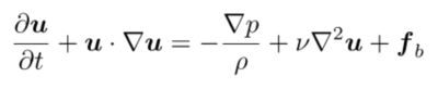
Where p is the static pressure, v is the viscosity and ƒb are body forces (typically gravity).
3. Conservation of Energy: First Law of Thermodynamics
The energy equation states that the change in total energy of the fluid must be equal to the energy added to, or removed from, the system (e.g. by conductive or convective heat transfer).
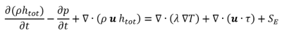
Where htot is the total enthalpy, λ is the conductivity, T the temperature and SE is external sources of energy. The term ∇ ∙ ( u ∙ t ) is the viscous work term and represents the work due to viscous stresses
Advancements in CFD
The potential of CFD is limited only by the power of computing hardware. As hardware and software advancements enable the transition of scientific computations from CPUs to GPUs, including applying multiple GPUs for CFD simulations, massive leaps in speed and accuracy are possible. Fully native multi-GPU implementations will further accelerate CFD simulations, fueling new performance levels, reducing hardware costs, and reducing power consumption.
Related Resources
See What Ansys Can Do For You
See What Ansys Can Do For You
Contact Us
Contact us today