


ANSYS BLOG
December 18, 2023
Using the Henyey-Greenstein Distribution Model to Visualize Bulk Scattering with OpticStudio
The Henyey-Greenstein model describes the angular distribution of light scattered by small particles. This model has been applied to numerous situations, ranging from the scattering of light by biological tissue to scattering by interstellar dust clouds.
Let's learn how to use a user-defined object (DLL file) to model Henyey-Greenstein bulk scattering in nonsequential mode below.
Understanding the Henyey-Greenstein Bulk Scatter Model
In the Henyey-Greenstein model, the angular distribution of scattered light is given by the following equation:
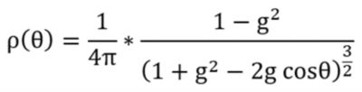
Henyey-Greenstein Model
The parameter g characterizes the distribution. For g=0, the model describes a material with a uniform probability of scattering at all angles, and as g approaches unity, the distribution becomes highly peaked around θ=0 degrees. The angle θ is defined as the angle of the scattered ray concerning the specular ray; θ=0 degrees refers to scattering along the specular ray in the forward direction, and θ=180 degrees to scattering along the specular ray in the backward direction.
A user-defined DLL is included with the Ansys Zemax OpticStudio installation and allows users to apply this bulk scattering model to any nonsequential volume. We will use the "Henyey-Greenstein-bulk.dll" in the example below to show the angular and power distribution of the Henyey-Greenstein model.
Examining the Distribution of Power in the Henyey-Greenstein Model
Let’s look at an example illustrating the implementation of the Henyey-Greenstein model in OpticStudio. This system consists of a source ray launching rays at normal incidence to a rectangular volume to which the Henyey-Greenstein scattering distribution has been applied. This distribution is applied to the volume by specifying a user-defined DLL.
The settings in Object Properties > Volume Physics in OpticStudio control what type of bulk scattering model to apply to the rectangular volume. In this example, the "model" is DLL Defined Scattering, and the selected DLL file is “Henyey-Greenstein-bulk.dll." This DLL and the corresponding source code are located in the folder "{Zemax}\DLL\BulkScatter."
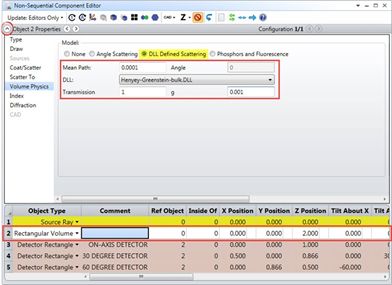
Figure 1. The Henyey-Greenstein-bulk.DLL.
Inputs to the DLL are the "Transmission" (which describes how much of the input power is attenuated during scattering) and the parameter g from the equation above. To measure scattered rays at various angles, three small detectors have been placed a uniform distance away from the volume in the example system at angles of 0, 30, and 60 degrees concerning the incident ray angle (see Figure 2).
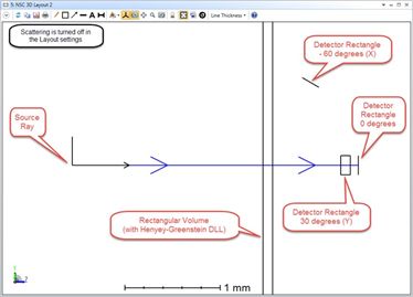
Figure 2. NSC 3D Layout without scattering turned on.
Note that Figure 2 shows the NSC 3D Layout tool without scattering turned on, so we’re only seeing the specular path. Before analyzing the results with scattering turned on, we can expand to see Object Properties > Source for the source ray. You will notice that the system has been set up to explicitly provide only one instance of scattering per incident ray in Figure 3.
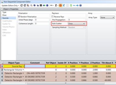
Figure 3. Show where to change the bulk scatter to once.
The default Bulk Scatter setting in OpticStudio is "Many," which means that the rays may scatter multiple times within the media. If “Once” is selected, each branch of a ray can only bulk scatter once. If a ray splits before scattering — at the interface of the scattering volume, for example — then each of the child rays may scatter, since each child’s branch is scattering for the first time. If “Never” is selected, then no bulk scattering will occur for rays from this source.
Scattering can be observed in the NSC 3D Layout tool by checking the “Scatter NSC Rays” box in Layout Settings (see Figure 4).
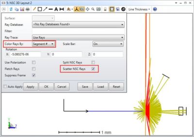
Figure 4. Shows the scattering that can be observed in the NSC 3D Layout tool.
Many of the rays miss the detectors, and these rays are only drawn a short distance to show their direction. To change the distance these rays are drawn, see the “Missed Ray Draw Distance” box under System Explorer > Non-Sequential in Figure 5.
This parameter is the distance to draw the ray segments that miss all objects. If zero, OpticStudio will select a default value for this parameter when drawing missed rays.
We can use filter strings to analyze only the rays, which scatter in the rectangular volume and hit the detector rectangle. The filter string defines a “test” that rays must pass before they are drawn or displayed. The filter string syntax consists of logical operations between commands or flags that indicate if the ray has hit, missed, reflected, refracted, scattered, diffracted, or ghost-reflected from an object.
A full list of filter string commands can be found in the OpticStudio Help Files.
Here are the flags we will use:
- Bn: shows rays that bulk scattered inside of object n.
- Hn: shows rays that hit object n.
- We can combine these filter strings using the following operators:
- &: logical AND. Both flags on either side of the “&” symbol must be TRUE for the AND operation to return TRUE.
- |: logical OR. If either of the flags are TRUE, OR returns TRUE.
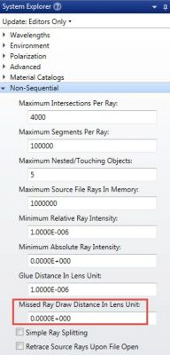
Figure 5. Shows if missed ray draw is zero, OpticStudio will select a default value for this parameter when drawing missed rays.
Therefore, to show rays that were bulk-scattered within the rectangular volume (object 2) and hit one of the detectors (objects 3, 4, and 5) we can use the filter string "B2 & (H3 | H4 | H5)." This filter string may be applied to layout rays in the NSC 3D Layout tool or the shaded model (see Figure 6).

Figure 6. Filter string may be applied to Layout rays in the NSC 3D Layout or the Shaded Model.
Filter strings may be applied to Analysis Rays in the “Ray Trace Control” window when the results are saved to Ray Database.
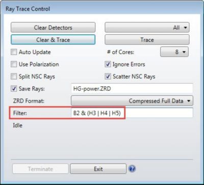
Figure 7. Shows how Filter strings may be applied to Analysis Rays in the Ray Trace Control.
The distribution of power landing on each detector is then measured for a case in which 5,000,000 analysis rays are launched with a total power of 1 W (and a transmission factor of unity). The results for g=0.001 and g=0.5 are shown in the table below.
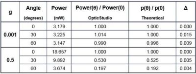
The "Mean Path” setting (mean free path) was specified as 0.0001 mm, which is small relative to the 0.1-mm thickness of the volume. The measured OpticStudio values reproduce those results derived from the theoretical model within statistical error, as we would expect for a case in which each ray is only allowed to scatter once (the results will vary from ray trace to ray trace due to statistics, so you will get different — but very similar — numbers).
To try out Ansys Zemax capabilities, download a free trial.
Note: If g=0 is specified as an input, the actual value of g used in the calculations is 10-4. This is due to a singularity in the calculations which arises when g=0. Results obtained for very small values of g are nearly identical to those expected for g=0, indicating that this approximation is sufficiently accurate.
See What Ansys Can Do For You
See What Ansys Can Do For You
Contact Us
Contact us today