


ANSYS BLOG
January 2, 2024
How to Determine the Resolution of Diffraction-limited Imaging Systems Using the Point Spread Function in Ansys Zemax OpticStudio
You can characterize the resolution of a diffraction-limited imaging system, such as a microscope, in many different ways. In Ansys Zemax OpticStudio, you can use the point spread function (PSF) for this purpose.
How imaging systems perform relates to their resolution, but the definition of resolution varies. In super-resolution microscopy, we can use the Fourier ring correlation to evaluate the resolution. In diffraction-limited microscopes, we can estimate the resolution with the Rayleigh criterion, also known as Sparrow’s criterion. In practice, the resolution of these systems can also be measured with microbeads, chosen to be significantly smaller than the expected resolution and assuming one of the above criterions. These microbeads act as point emitters that form a PSF. The size of the beads gives an estimate of the resolution in the image.
Method 1: Multiconfiguration Editor (Coherent Imaging)
For the purposes of this blog, we will use a microscope design based on a TL4X-SAP objective lens (4X, 0.2 NA), and a TTL200 tube lens (Figure 1). Both lenses are available as black boxes from THORLABS website.
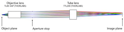
Figure 1. Microscope design composed of black box elements from THORLABS. The magnification is 4X and numerical aperture (NA) is 0.2.
We will use the “Real Image Height” field definition in OpticStudio and specify five fields with equal areas over a square of X, and Y half-width of 6.656 mm, corresponding to 1.664 mm in the object plane. The field definition models a scientific complementary metal-oxide semiconductor (sCMOS) detector with 2048 x 2048 pixels and a physical size of 13.312 by 13.312 mm2 in the image plane. These detectors are commonly used in microscopy and can be found in products such as the Hammamatsu Orca-Flash4.0 V3 and Andor Zyla 4.2 PLUS cameras.
We are also using the wavelength F, d, C (Visible) preset in OpticStudio. The optimization is performed using the criterion “RMS Wavefront Centroid” with four rings and six arms, and will use default air boundary constraints (0-1,000 mm). Additionally, the system will be constrained for telecentricity and -4X magnification. (In this microscope design, the image is reversed.)
We have chosen this microscope design because it is relatively easy to set up and has real-life applications. For example, telecentricity is often required in machine vision applications. We have kept the optimization simple, and the results and conclusions will apply to most imaging systems with conjugated object and image planes.
Multiconfiguration Setup
To address the resolution of the microscope design, we will create two point sources at the object plane, which we will gradually separate with a distance close to the Rayleigh criterion. We will observe how their PSFs overlap in the image plane. In the microscope design, the Rayleigh criterion yRayleigh is calculated as:

In which λPrimary is the primary wavelength (0.588 um) and NA is the numerical aperture of the objective lens (0.2). While the Rayleigh criterion can serve as a measure of the system resolution, it assumes a perfectly circular, unaberrated aperture stop and incoherent illumination. Additionally, the Rayleigh criterion is a subjective metric to establish the discernability of two PSFs, which depends on the observer, and the kind of information which needs to be retrieved from the microscope images.
We will start by removing all but the on-axis field (Field 1) will convert it to "Object Height" (Figure 2).
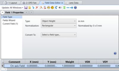
Figure 2. Field setup for the Multiconfiguration method to analyze microscope resolution. Only the on-axis field is kept, and it has been converted to “Object Height.”
Then, we will create two configurations with a single “YFIE” operand, and we will specify a value of 1.8e-3 mm in the second configuration (see Figure 3).

Figure 3. Multiconfiguration setup for the PSF overlap analysis. The two point sources are separated by 1.8 um in the object plane.
Finally, we use the “Huygens PSF” and “Huygens PSF Cross-section” tools to analyze the overlap of the two PSFs in the image plane. Those two analyses can perform a coherent sum of the individual PSFs across the two configurations (see the Help File for more details).
See Figure 4 for the analysis’ settings. The Multiconfiguration setting is shown with a red box and arrow. (Note: This option is not available with the FFT PSF tool.)
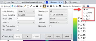
Figure 4. Huygens PSF settings. By checking all configurations from the menu bar, we can obtain the coherent sum of the individual PSFs.
We’re focusing the resolution analysis on the on-axis field, but the same analysis can be conducted for every part of the field.
The results of the Huygens PSF analysis are shown in Figure 5.
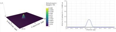
Figure 5. Results of the Huygens PSF and PSF Cross-section overlap with an object plane Y-field separation of 1.8 um (Rayleigh criterion) in multiple configurations. The two point sources are hardly distinguishable by eye in this microscope design.
As you can see, the two field points severely overlap in the image plane, and their respective PSFs are nearly undistinguishable. There are two reasons for this result. First, by performing a coherent sum of the PSFs, the incoherent illumination assumption of the Rayleigh criterion is violated, which causes the resolution to degrade. Second, the OPD Fan shows aberrations in the order of 0.25 waves, and this microscope sits at the edge of the diffraction limit. This means it is sufficiently diffraction limited to allow for analyses such as Huygens PSF, but it still presents some geometric aberrations, which alters the diffraction-limited performance of the system.
From the Rayleigh criterion, we can increase the separation distance of the fields and reevaluate the results. We did this in Figure 6, with a separation of 2.3 um in object plane.

Figure 6. Results of the Huygens PSF and PSF Cross-section overlap with an object plane Y-field separation of 2.3 um in multiple configurations. By increasing the separation distance between the field points, the PSFs start to separate in the image plane and you can observe two distinct peaks.
With a greater field separation, the resulting PSFs become distinguishable. The peak separation in the Huygens PSF Cross-section is almost 10 um, which is in agreement with the system magnification (4X). (When we say "distinguishable," we mean a qualitative assessment of what we see in Figure 6 — however, this criterion can be made more objective if we define how the peaks should be separated in terms of post-processing, which is out of the scope of this tutorial.)
Lastly, we can account for the physical pixel size of our detector to get an image as seen from the microscope. The PSFs have a full width at half-maximum of approximately 12 um, and our hypothetic detector has a physical pixel size of 6.5 um. This clearly violates Nyquist-Shanon's sampling theorem, which is yet another limitation of the microscope design. Figure 7 shows the Huygens PSF analysis results when the image sampling is changed to 32 x 32 pixels with an image delta (the physical pixel size) set to 6.5 um.

Figure 7. PSFs overlap when accounting for the physical pixel size of the detector. Too few pixels compose the PSF overlap and further degrade the resolution of the microscope.
As you can see, the inadequate physical pixel size further degrades the resolution of the microscope. While the two peaks were distinguishable in Figure 6, they are now overlapping again in Figure 7. In this case, the microscope resolution is said to be pixel limited and is given by at least twice the pixel size scaled by the magnification, meaning 3.25 um (two times 6.5 divided by 4). The result of a 3.25 um separation distance between the fields in object plane is depicted in Figure 8.

Figure 8. PSFs overlap when accounting for the physical pixel size of the detector. A separation of 3.25 um allows to separate the close fields again. This distance corresponds to twice the pixel size divided by the magnification — a consequence of Nyquist-Shanon's sampling theorem.
By accounting for the detector pixel size, a greater separation is needed to avoid PSF aliasing and ensure it is represented by at least 2 pixels. The field separation of 3.25 um is quite different from the 1.8 um Rayleigh criterion, and this shows just how ambiguous the definition of resolution can be. We have also not considered the tolerancing of the microscope, which would further reduce this metric.
The method presented in this section considered the coherent sum of two nearby PSFs and showed how these could be distinguished from one another. While this method is suited to coherent imaging systems, it is generally more conservative for incoherent imaging systems. This could lead to overperforming designs, which are inherently more costly. For example, in fluorescence microscopy, the resolution is measured with fluorescent microbeads, the light from which is often considered incoherent. In this case, the performance of the microscope is expected to be more in line with the Rayleigh criterion.
In the next section, we show how to use the Image Simulation feature of OpticStudio to investigate the microscope design’s resolution under the incoherent illumination assumption by incoherently summing PSFs from closely located field points.
Method 2: Image Simulation (Incoherent Imaging)
For this method, we can keep the original microscope design with its five field points. We can convert those to Object Height (Figure 2). (For more details about the Image Simulation tool, see this Knowledgebase article.)
The first step to set up the Image Simulation is to provide it with an input image file. Since Image Simulation essentially performs a convolution of the microscope PSF with this input image, we want to have a Kronecker delta in the input image to model closely separated fields. In other words, the input image is a completely black (i.e., zero-valued pixels) background, with a single white (maximum-valued) pixel at the position of each field. The size of the pixels is made as small as possible while keeping the image size, which leads to decent computation time in the order of minutes.
We choose to represent approximately four times the area of the Huygens PSF presented in Figures 5-8 (400 x 400 um2), which makes for an intrinsic guard band. This area is scaled to correspond to a field size of 100 by 100 um2. We also chose the image size to be 1,600 by 1,600 pixels; hence, the pixel dimension is 0.0625 by 0.0625 um2, well below the Rayleigh criterion of 1.8 um. We create six white pixels in the image that correspond to three cases of two nearby fields. The three cases are approximately the same as what was investigated in the first method: 1.8 (29), 2.3 (37), and 3.25 (52) um, respectively. A zoomed-in region of the input image containing the white pixels is shown in Figure 9.
Figure 9. Zoomed-in input image showing the six white pixels corresponding to three pairs of field. The vertical separation is 6.25 (100) um (pixels) and avoids overlap between the field pairs. The upper pixel in the middle is located at coordinate (800, 800) in the image.
The Source Bitmap Settings of Image Simulation are shown in Figure 10.
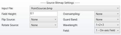
Figure 10. Image Simulation settings for the Source Bitmap. The field height is 100 um (0.1 mm in lens units), and the input image is centered on the On-axis Field.
The Field Height is 100 um. We also focus the analysis on the On-axis Field for this method, but the same analysis can also be conducted at different field positions. We use the combination of wavelengths 1 to 3, currently defined in the System Explorer.
The PSF grid settings are shown in Figure 11.
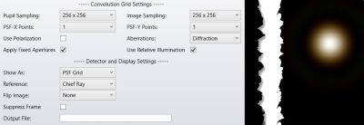
Figure 11. Left: Convolution Grid Settings in the Image Simulation feature. It uses a single PSF on-axis due to the restricted field where the analysis is conducted. The sampling settings are chosen the same as for the Huygens PSF method. Aberrations are set to Diffraction. Right: Resulting PSF grid in the Image Simulation feature.
We use the same sampling settings as the Huygens PSF method and a single PSF on-axis. We are doing so because the Field Height is set to 100 um. The results of running the Image Simulation feature are shown in Figure 12.
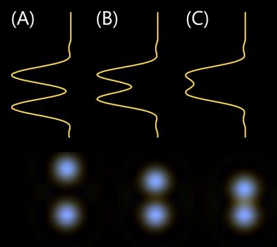
Figure 12. Image Simulation results with default Detector and Display Settings (all zero). The first row depicts the intensity profile across the center line going through both PSFs, and the second row is the Image Simulation output for (A) 3.25, (B) 2.3, and (C) 1.8 um separation between the fields. The image is reversed due to the optical property of the microscope (negative magnification).
From Figure 12 (C), we can observe that a separation of 1.8 um, the Rayleigh criterion, makes the two PSFs distinguishable. There is a small dip of approximately 15% in intensity, which we can use to post-process the image with a threshold, for example. The greater the distance between the fields, the better the separation.
When compared to the Huygens PSF method, which uses the coherent sum of PSFs across configurations, the results are better in terms of resolvability of the PSFs. However, we have not considered the physical size of the detector yet. We can adjust the Image Simulation settings to match Figure 13 to account for the detector characteristics.
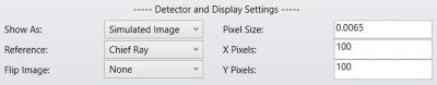
Figure 13. Detector and Display Settings when considering the physical size of the microscope detector.
The result of accounting for the detector physical properties is shown in Figure 14.

Figure 14. Image Simulation results accounting for the physical size of the microscope detector. Even a separation of 3.25 um in the object plane does not separate the PSFs. The vertical separation of 6.25 um makes the field pairs distinguishable.
The separation between closely located fields is no longer possible, and you can observe that strictly using Nyquist-Shannon sampling theorem to determine the pixel-limited resolution is not sufficient. The vertical separation between the field pairs is 6.25 um in the object plane (Figure 9) and makes for a clean separation between those pairs. Therefore, we assume the resolution is between 3.25 and 6.25 um. Further investigation shows that separation of 5.125 um gives a visual qualitative separation of the source points, as shown in Figure 15.
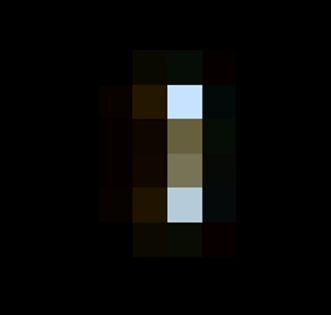
Figure 15. Image Simulation results for a pair of points separated by 5.125 um in the object plane. Two brighter pixels seem to be qualitatively distinguishable.
For more articles like this, visit our Knowledgebase.
Try Ansys optical design software capabilities for yourself by requesting a free trial today.
References
- N. Banterle, K. HuyBui, E. A.Lemke, and M. Beck, "Fourier ring correlation as a resolution criterion for super-resolution microscopy," J. Struct. Biol 183 (3), pp 363-367 (2013)
- J. S. Silfies, and S. A. Schwartz, "The Diffraction Barrier in Optical Microscopy," Retrieved from: https://www.microscopyu.com/techniques/super-resolution/the-diffraction-barrier-in-optical-microscopy on November 12, 2019.
See What Ansys Can Do For You
See What Ansys Can Do For You
Contact Us
Contact us today